If you work with network data, and especially with a lot of (small) networks, you might be interested in the rgraph6 package that just made it to CRAN. It implements methods to encode and decode graphs as strings of printable ASCII characters using formats graph6, digraph6 and sparse6. The formats themselves are due to Brendan McKay and are described in the paper by McKay and Piperno (2014) and on this page.
Tl;dr, you can store a collection of graphs as an R character vector, elments of which consist of letters and other printable characters.
I have developed first prototypes of the functions handling the graph6 format while working on a simulation study for a chapter of my PhD thesis (published as Bojanowski and Buskens 2011). In short, the simulation required sampling an initial network and running a certain dynamic process until it reaches an equilibrium state, and this 300k times. It was of interest to store both the initial and final (equlibrium) network together with their selected topological properties. The ‘graph6’ format was perfect for that task (hat tip Vincent Buskens). This was over 15 years ago, so as such this package is an instance of dusting-off some code from the drawer.
Thanks to non-trivial contributions by David (@schochastics) the package now handles the three formats (‘graph6’, ‘digraph6’ and ‘sparse6’) and allows for encoding and decoding to/from igraph objects (Csardi and Nepusz 2006), network objects (Butts 2015, 2008), adjacency matrices and edgelist matrices.
The formats
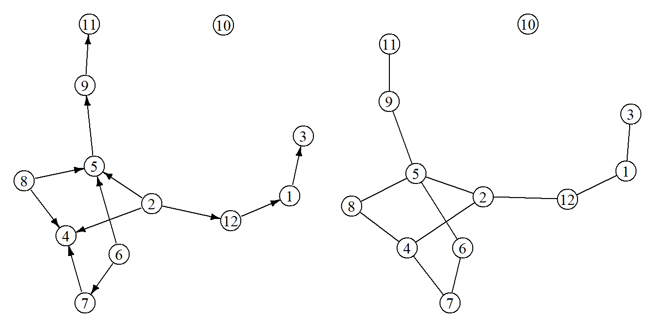
To show the formats let’s generate a directed (g_directed) and undirected (g_undirected) graphs:
library(igraph)
set.seed(123)
g_directed <- sample_gnm(12, 12, directed=TRUE)
g_undirected <- as.undirected(g_directed)
Figure 1: Example networks.
Digraph6
The ‘digraph6’ format is designed for directed graphs. Encoding g_directed will give:
library(rgraph6)
as_digraph6(g_directed)
## [1] "&KG?E@?????GA_C?E??A????_?"Graph6
The ‘graph6’ format is designed for undirected graphs. It should be more efficient for dense graphs. Encoding g_undirected will give:
as_graph6(g_undirected)## [1] "KQOGgoG??@W?"Sparse6
The ‘sparse6’ format is designed for undirected graphs. It should be more efficient for sparse graphs. Encoding g_undirected will give:
as_sparse6(g_undirected)## [1] ":KcAKYRJKdLG_F"Main functions
Main functions for encoding network data are:
graph_as_text()– the format will be chosen automatically.as_graph6()as_sparse6()as_digraph6()
Main functions for decoding are:
adjacency_from_text()edgelist_from_text()igraph_from_text()network_from_text()
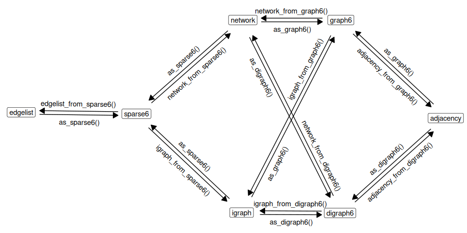
Implemented functions are shown on the following graph:

Figure 2: Diagram of functions implemented in the ‘rgraph6’ package
More examples
Encode a list of ‘igraph’ objects
Let’s generate a list of igraph objects:
set.seed(666)
igraph_list <- replicate(5, igraph::sample_gnp(10, 0.1, directed=FALSE),
                         simplify = FALSE)
Encode as a vector of ‘graph6’ symbols:
as_graph6(igraph_list)## [1] "ICG_@?W??" "I????@B?G" "I?@O????W" "I@@A?E???" "I?_?_@_??"Encode as a vector of ‘sparse6’ symbols:
as_sparse6(igraph_list)## [1] ":IeASjaeR" ":IoCp{^" ":IiC]Rg" ":IeIgWu`" ":IgAo{@D"Decode a vector of different types of symbols
The package provides example data g6, d6, and s6. Let’s create a short vector with a mixture of ‘graph6’, ‘digraph6’ and ‘sparse6’ symbols:
x <- c(g6[1], s6[2], d6[3])
x
## [1] "N??E??G?e?G?????GGO"
## [2] ":NkF?XduSqiDRwYU~"
## [3] "&N?R_?E?C?D??U_A????????O???????????????"Decode it to a list of igraph objects:
igraph_from_text(x)## [[1]]
## IGRAPH 59d2f61 U--- 15 10 --
## + edges from 59d2f61:
## [1] 1-- 7 1--11 2-- 7 2--11 2--12 2--15 5-- 9 7--10 8--15 13--15
##
## [[2]]
## IGRAPH 59d2a80 U--- 15 13 --
## + edges from 59d2a80:
## [1] 2-- 7 2-- 9 4--10 6--10 6--12 7--12 11--12 5--13 6--13 10--13
## [11] 4--15 10--15 14--15
##
## [[3]]
## IGRAPH 59d31d4 D--- 15 15 --
## + edges from 59d31d4:
## [1] 1-> 8 1->11 1->12 1->13 2->13 2->14 3->10 4-> 7 4-> 9 5-> 8 5->10 5->11
## [13] 5->13 6-> 8 9->14Decode it to a list of network objects:
network_from_text(x)## Loading required namespace: network## [[1]]
## Network attributes:
## vertices = 15
## directed = FALSE
## hyper = FALSE
## loops = FALSE
## multiple = FALSE
## bipartite = FALSE
## total edges= 10
## missing edges= 0
## non-missing edges= 10
##
## Vertex attribute names:
## vertex.names
##
## No edge attributes
##
## [[2]]
## Network attributes:
## vertices = 15
## directed = FALSE
## hyper = FALSE
## loops = FALSE
## multiple = FALSE
## bipartite = FALSE
## total edges= 13
## missing edges= 0
## non-missing edges= 13
##
## Vertex attribute names:
## vertex.names
##
## No edge attributes
##
## [[3]]
## Network attributes:
## vertices = 15
## directed = TRUE
## hyper = FALSE
## loops = FALSE
## multiple = FALSE
## bipartite = FALSE
## total edges= 15
## missing edges= 0
## non-missing edges= 15
##
## Vertex attribute names:
## vertex.names
##
## No edge attributesTidy graph databases (base R)
The formats shine if we need to store large number of graphs in a data frame / tibble. Let’s generate a list of random graphs as igraph objects and store them in a data frame column of ‘graph6’ symbols:
set.seed(666)
d <- data.frame(
  gr6 = as_graph6(replicate(
    10,
    random.graph.game(sample(3:12, replace=TRUE), p=.5, directed=FALSE),
    simplify=FALSE
  ))
)
d
## gr6
## 1 FblF_
## 2 DFc
## 3 HfTaMwk
## 4 KefToktrftZ~
## 5 JPraDzZQ?M?
## 6 Bo
## 7 Ed`w
## 8 Gpuq|{
## 9 EbSG
## 10 ICNa@Gg\\oNice and compact. We can go further by doing some computations and saving the results together with the graph data. Let’s add number of edges, vertices and the density:
d2 <- within(
  d, {
    igraphs <- igraph_from_text(gr6)
    vc <- vapply(igraphs, vcount, integer(1))
    ec <- vapply(igraphs, ecount, numeric(1))
    density <- vapply(igraphs, edge_density, numeric(1))
})
d2$igraphs <- NULL # drop the list column with igraph objects
d2
## gr6 density ec vc
## 1 FblF_ 0.5238095 11 7
## 2 DFc 0.5000000 5 5
## 3 HfTaMwk 0.5000000 18 9
## 4 KefToktrftZ~ 0.6212121 41 12
## 5 JPraDzZQ?M? 0.4363636 24 11
## 6 Bo 0.6666667 2 3
## 7 Ed`w 0.5333333 8 6
## 8 Gpuq|{ 0.6785714 19 8
## 9 EbSG 0.4000000 6 6
## 10 ICNa@Gg\\o 0.3777778 17 10This can be to a simple CSV file
write.csv(d2, row.names = FALSE)## "gr6","density","ec","vc"
## "FblF_",0.523809523809524,11,7
## "DFc",0.5,5,5
## "HfTaMwk",0.5,18,9
## "KefToktrftZ~",0.621212121212121,41,12
## "JPraDzZQ?M?",0.436363636363636,24,11
## "Bo",0.666666666666667,2,3
## "Ed`w",0.533333333333333,8,6
## "Gpuq|{",0.678571428571429,19,8
## "EbSG",0.4,6,6
## "ICNa@Gg\o",0.377777777777778,17,10Detaching igraph to avoid conflicts:
detach(package:igraph)Tidy graph databases (tidyverse)
The same operations as above, but using tidyverse (Wickham et al. 2019) functions and tibbles:
library(dplyr)##
## Attaching package: 'dplyr'## The following objects are masked from 'package:stats':
##
## filter, lag## The following objects are masked from 'package:base':
##
## intersect, setdiff, setequal, unionset.seed(666)
d <- tibble(
gr6 = as_graph6(replicate(
10,
igraph::random.graph.game(sample(3:12, replace=TRUE), p=.5, directed=FALSE),
simplify=FALSE
))
)
d## # A tibble: 10 x 1
## gr6
## <chr>
## 1 "FblF_"
## 2 "DFc"
## 3 "HfTaMwk"
## 4 "KefToktrftZ~"
## 5 "JPraDzZQ?M?"
## 6 "Bo"
## 7 "Ed`w"
## 8 "Gpuq|{"
## 9 "EbSG"
## 10 "ICNa@Gg\\o"d2 <- d %>%
mutate(
igraphs = igraph_from_text(gr6),
vc = vapply(igraphs, igraph::vcount, integer(1)),
ec = vapply(igraphs, igraph::ecount, numeric(1)),
density = vapply(igraphs, igraph::edge_density, numeric(1))
)
d2## # A tibble: 10 x 5
## gr6 igraphs vc ec density
## <chr> <list> <int> <dbl> <dbl>
## 1 "FblF_" <igraph> 7 11 0.524
## 2 "DFc" <igraph> 5 5 0.5
## 3 "HfTaMwk" <igraph> 9 18 0.5
## 4 "KefToktrftZ~" <igraph> 12 41 0.621
## 5 "JPraDzZQ?M?" <igraph> 11 24 0.436
## 6 "Bo" <igraph> 3 2 0.667
## 7 "Ed`w" <igraph> 6 8 0.533
## 8 "Gpuq|{" <igraph> 8 19 0.679
## 9 "EbSG" <igraph> 6 6 0.4
## 10 "ICNa@Gg\\o" <igraph> 10 17 0.378# Show-off the CSV
d2 %>%
select(- igraphs) %>%
readr::write_csv(file=stdout())## gr6,vc,ec,density
## FblF_,7,11,0.5238095238095238
## DFc,5,5,0.5
## HfTaMwk,9,18,0.5
## KefToktrftZ~,12,41,0.6212121212121212
## JPraDzZQ?M?,11,24,0.43636363636363634
## Bo,3,2,0.6666666666666666
## Ed`w,6,8,0.5333333333333333
## Gpuq|{,8,19,0.6785714285714286
## EbSG,6,6,0.4
## ICNa@Gg\o,10,17,0.37777777777777777