In data analysis it happens sometimes that it is neccesary to use weights. Contexts that come to mind include:
- Analysis of data from complex surveys, e.g. stratified samples. Sample inclusion probabilities might have been unequal and thus observations from different strata should have different weights.
- Application of propensity score weighting e.g. to correct data being Missing At Random (MAR).
- Inverse-variance weighting (https://en.wikipedia.org/wiki/Inverse-variance_weighting) when different observations have been measured with different precision which is known apriori.
- We are analyzing data in an aggregated form such that the weight variable encodes how many original observations each row in the aggregated data represents.
- We are given survey data with post-stratification weights.
If you use, or have been using, SPSS you probably know about the possibility to define one of the variables as weights. This information is used when producing cross-tabulations (cells include sums of weights), regression models and so on. SPSS weights are frequency weights in the sense that \(w_i\) is the number of observations particular case \(i\) represents.
On the other hand, in R lm() and glm() functions have weights argument that serves a related purpose.
suppressMessages(local({
  library(dplyr)
  library(ggplot2)
  library(survey)
  library(knitr)
  library(tidyr)
  library(broom)
}))
Let’s compare different ways in which a linear model can be fitted to data with weights. We start by generating some artificial data:
set.seed(666)

N <- 30 # number of observations

# Aggregated data
aggregated <- data.frame(x = 1:5) %>%
  mutate(
    y = round(2 * x + 2 + rnorm(length(x)) ),
    freq = as.numeric(table(
      sample(1:5, N, replace=TRUE, prob=c(.3, .4, .5, .4, .3))
    ))
  )
aggregated
## x y freq
## 1 1 5 4
## 2 2 8 5
## 3 3 8 8
## 4 4 12 8
## 5 5 10 5# Disaggregated data
individuals <- aggregated[ rep(1:5, aggregated$freq) , c("x", "y") ]Visually:
ggplot(aggregated, aes(x=x, y=y, size=freq)) +
  geom_point() +
  theme_bw()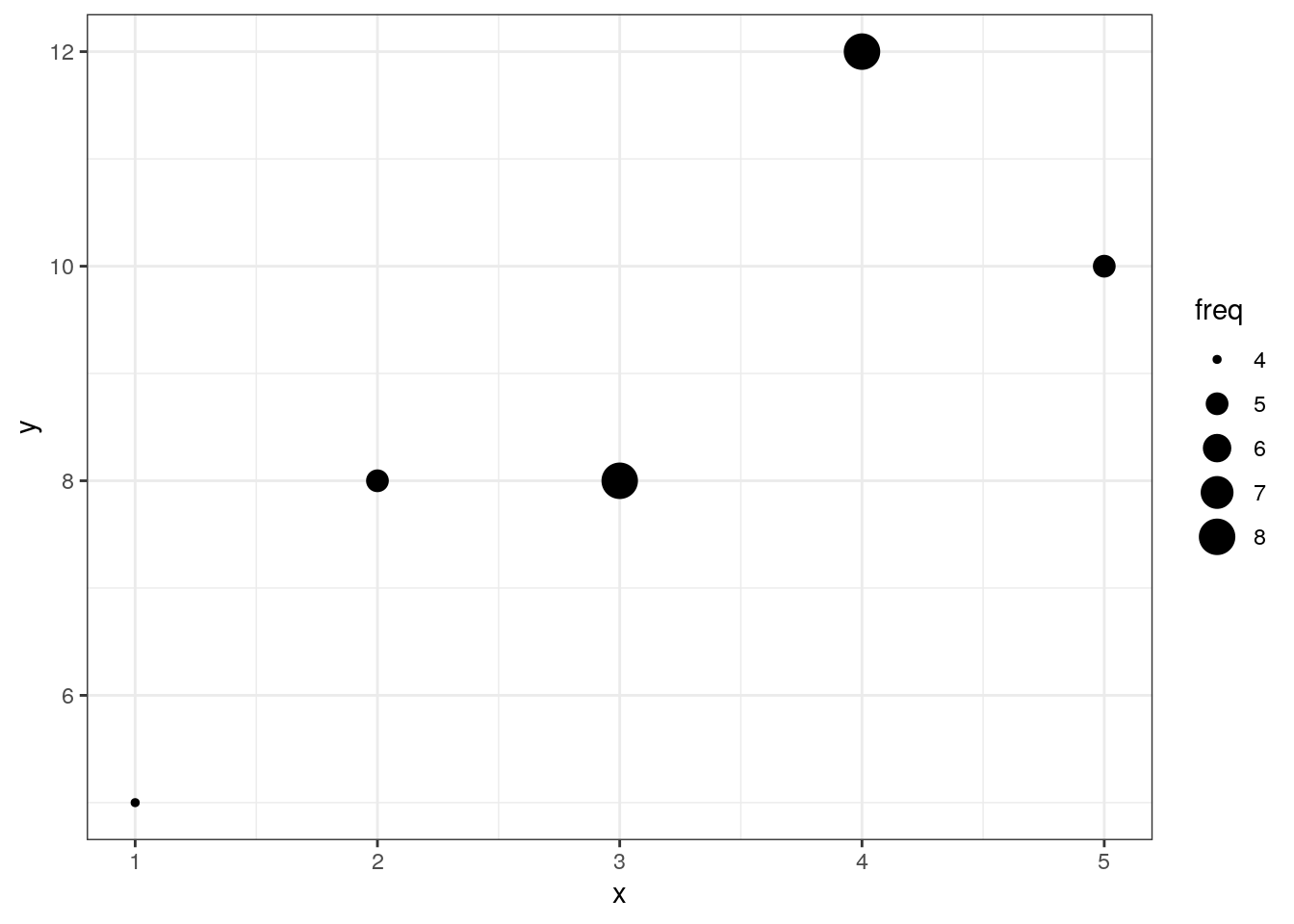
Let’s fit some models:
models <- list(
  ind_lm = lm(y ~ x, data=individuals),
  raw_agg = lm( y ~ x, data=aggregated),
  ind_svy_glm = svyglm(y~x, design=svydesign(id=~1, data=individuals),
                       family=gaussian() ),
  ind_glm = glm(y ~ x, family=gaussian(), data=individuals),
  wei_lm = lm(y ~ x, data=aggregated, weight=freq),
  wei_glm = glm(y ~ x, data=aggregated, family=gaussian(), weight=freq),
  svy_glm = svyglm(y ~ x, design=svydesign(id=~1, weights=~freq, data=aggregated),
                   family=gaussian())
)
## Warning in svydesign.default(id = ~1, data = individuals): No weights or
## probabilities supplied, assuming equal probabilityIn short, we have the following linear models:
ind_lmis a OLS fit to individual data (the true model).ind_aggis a OLS fit to aggregated data (definitely wrong).ind_glmis a ML fit to individual dataind_svy_glmis a ML fit to individual data using simple random sampling with replacement design.wei_lmis OLS fit to aggregated data with frequencies as weightswei_glmis a ML fit to aggregated data with frequencies as weightssvy_glmis a ML fit to aggregated using “survey” package and using frequencies as weights in the sampling design.
We would expect that models ind_lm, ind_glm, and ind_svy_glm will be identical.
Summarise and gather in long format
results <- models %>%
  lapply(tidy) %>%
  bind_rows(.id = "model")
Check if point estimates of model coefficients are identical:
results %>%
  pivot_wider(model, names_from="term", values_from = "estimate") %>%
knitr::kable()| model | (Intercept) | x |
|---|---|---|
| ind_lm | 4.33218 | 1.474048 |
| raw_agg | 4.40000 | 1.400000 |
| ind_svy_glm | 4.33218 | 1.474048 |
| ind_glm | 4.33218 | 1.474048 |
| wei_lm | 4.33218 | 1.474048 |
| wei_glm | 4.33218 | 1.474048 |
| svy_glm | 4.33218 | 1.474048 |
Apart from the “wrong” raw_agg model, the coefficients are identical across models.
Let’s check the inference:
# Standard Errors
results %>%
  pivot_wider(model, names_from="term", values_from = "std.error") %>%
knitr::kable()| model | (Intercept) | x |
|---|---|---|
| ind_lm | 0.652395 | 0.1912751 |
| raw_agg | 1.669331 | 0.5033223 |
| ind_svy_glm | 0.500719 | 0.1912161 |
| ind_glm | 0.652395 | 0.1912751 |
| wei_lm | 1.993100 | 0.5843552 |
| wei_glm | 1.993100 | 0.5843552 |
| svy_glm | 1.221133 | 0.4926638 |
# p-values
results %>%
  pivot_wider(model, names_from="term", values_from = "p.value") %>%
knitr::kable()| model | (Intercept) | x |
|---|---|---|
| ind_lm | 0.0000003 | 0.0000000 |
| raw_agg | 0.0779371 | 0.0689035 |
| ind_svy_glm | 0.0000000 | 0.0000000 |
| ind_glm | 0.0000003 | 0.0000000 |
| wei_lm | 0.1180573 | 0.0859862 |
| wei_glm | 0.1180573 | 0.0859862 |
| svy_glm | 0.0381540 | 0.0580381 |
Recall, that the correct model is ind_lm. Observations:
raw_aggis clearly wrong, as expected.- Should the
weightargument tolmandglmimplement frequency weights, the results forwei_lmandwei_glmwill be identical to that fromind_lm. Only the point estimates are correct, all the inference stats are not correct. - The model using design with sampling weights
svy_glmgives correct point estimates, but incorrect inference. - Suprisingly, the model fit with “survey” package to the individual data using simple random sampling design (
ind_svy_glm) does not give identical inference stats to those fromind_lm. They are close though.
Functions weights lm and glm implement precision weights: inverse-variance weights that can be used to model differential precision with which the outcome variable was estimated.
Functions in the “survey” package implement sampling weights: inverse of the probability of particular observation to be selected from the population to the sample.
Frequency weights are a different animal.
However, it is possible get correct inference statistics for the model fitted to aggregated data using lm with frequency weights supplied as weights. What needs correcting is the degrees of freedom (see also http://stackoverflow.com/questions/10268689/weighted-regression-in-r).
models$wei_lm_fixed <- models$wei_lm
models$wei_lm_fixed$df.residual <- with(models$wei_lm_fixed, sum(weights) - length(coefficients))

results <- models %>%
  lapply(tidy) %>%
  bind_rows(.id = "model")
## Warning in summary.lm(x): residual degrees of freedom in object suggest this is
## not an "lm" fit# Coefficients
results %>%
pivot_wider(model, names_from="term", values_from = "estimate") %>%
knitr::kable()| model | (Intercept) | x |
|---|---|---|
| ind_lm | 4.33218 | 1.474048 |
| raw_agg | 4.40000 | 1.400000 |
| ind_svy_glm | 4.33218 | 1.474048 |
| ind_glm | 4.33218 | 1.474048 |
| wei_lm | 4.33218 | 1.474048 |
| wei_glm | 4.33218 | 1.474048 |
| svy_glm | 4.33218 | 1.474048 |
| wei_lm_fixed | 4.33218 | 1.474048 |
# Standard Errors
results %>%
  pivot_wider(model, names_from="term", values_from = "std.error") %>%
knitr::kable()| model | (Intercept) | x |
|---|---|---|
| ind_lm | 0.652395 | 0.1912751 |
| raw_agg | 1.669331 | 0.5033223 |
| ind_svy_glm | 0.500719 | 0.1912161 |
| ind_glm | 0.652395 | 0.1912751 |
| wei_lm | 1.993100 | 0.5843552 |
| wei_glm | 1.993100 | 0.5843552 |
| svy_glm | 1.221133 | 0.4926638 |
| wei_lm_fixed | 0.652395 | 0.1912751 |
See model wei_lm_fixed. Thus, correcting the degrees of freedom manually gives correct coefficient estimates as well as inference statistics.
Performance
Aggregating data and using frequency weights can save you quite some time. To illustrate it, let’s generate large data set in a disaggregated and aggregated form.
N <- 10^4

# Aggregated data
big_aggregated <- data.frame(x=1:5) %>%
  mutate(
    y = round(2 * x + 2 + rnorm(length(x)) ),
    freq = as.numeric(table(
      sample(1:5, N, replace=TRUE, prob=c(.3, .4, .5, .4, .3))
    ))
  )

# Disaggregated data
big_individuals <- aggregated[ rep(1:5, big_aggregated$freq) , c("x", "y") ]
… and fit lm models weighting the model on aggregated data. Benchmarking:
library(microbenchmark)

speed <- microbenchmark(
  big_individual = lm(y ~ x, data=big_individuals),
  big_aggregated = lm(y ~ x, data=big_aggregated, weights=freq)
)

speed %>%
  group_by(expr) %>%
  summarise(median=median(time / 1000)) %>%
  mutate( ratio = median / median[1])
## # A tibble: 2 x 3
## expr median ratio
## * <fct> <dbl> <dbl>
## 1 big_individual 4029. 1
## 2 big_aggregated 1667. 0.414So quite an improvement.
The improvement is probably the bigger, the more we are able to aggregate the data.